DESIGN OF EXPERIMENT
- sjhyun20
- Jan 24, 2022
- 6 min read
For this week's lesson, we were introduced to Design of Experiment (DOE). DOE is a statistics-based approach to designing experiments. It is a methodology to obtain knowledge of a complex, multi-variable process with the fewest trial possible. This is essential for engineering student, as we need to conduct hundreds and thousands of tests to determine factor effect for the most optimised output. DOE teaches us how to compute, analyse and interpret these data.
To evaluate our understanding on DOE, we were tasked to complete differnt case studies among our group.
For my case study, I had to do it based on a scenario where, in a wastewater treatment facility, a combination of coagulant chemicals, treatment temperature and stirring speed were identified as a critical factor to treat the wastewater to produce clean water. The clean water produced is recycled back into the main proses and at the same time reduce the amount of pollutant discharged by the plant.
8 runs were performed, and the data are shown below.
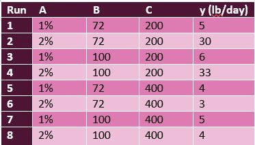
The response variable (y) is the amount of pollutant discharged (lb/day) with factors,
A = concentration of coagulant added, 1% and 2% by weight
B = treatment temperature, 72oF and 100oF
C = Stirring speed, 200 rpm and 400 rpm
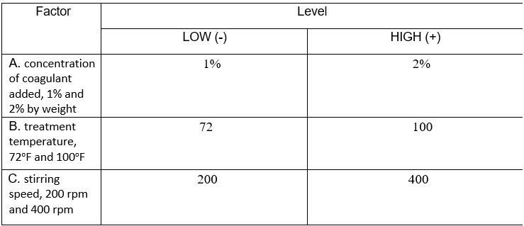
With the scenario all set, I started off DOE by indicating the high and low levels of the 3 factors.
‘+’ indicates the high level.
‘-‘ indicates the low level.
I then re-interpreted the 8 runs into a high and low level data.
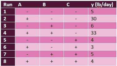
With all these complete, I could now start DOE. Both FULL factorial design and FRACTIONAL factorial design were performed for this case study.
FULL factorial run
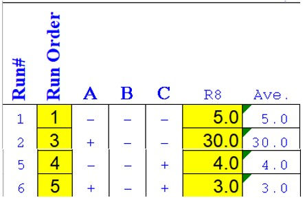
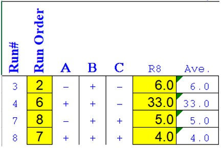
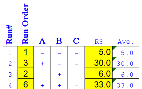
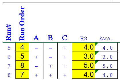
Firstly, the results were inputted into the DOE excel template, given to us on BlackBoard. Certain areas, such as the number of repeats, had to be removed as it was not coinciding with the case study. The final excel template is as shown below.

With all the values inputted, excel being the powerful software it is, it automatically computed the average significance on the mass of pollutant discharged as the 3 factors moved from the high to low level. I am then able to plot a graph with these values for easier comparison and to determine which factor has the most influence to the output. The graph is plotted in a way that the y-axis is the output and the x-axis are the changes of the 3 factors.
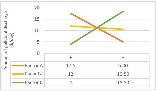
From the graph, we are able to interpret that Factor C contributes the most to the amount of pollutant discharged. It has the steepest curve and the biggest change of -14.50 as the stirrer speed changes from 400rpm to 200rpm. This suggests that as stirrer speed decrease, the amount of pollutant discharges increases by 14.50. Factor A contributes the second-most to the amount of pollutant discharged. It has the second-most steep curve and has a change of +12.50 as concentration of coagulant changes from 2% to 1%. This suggests that as concentration decreases, the amount of pollutant discharged decreases by 12.50. And lastly, Factor B contributes the least to the amount of pollutant discharged. It has an almost straight curve and the smallest change of +1.50 as temperature of treatment decreases from 100 oF to 72 oF. This suggests that as temperature decreases, the amount of pollutant discharged decreases by 1.50, which is less that when concentration changes.
As such, the final ranking is
Stirrer speed
Concentration of coagulant added
Treatment temperature
However, just the factors alone are not reliable enough to rank and determine which factor affects the amount of pollutant discharged the most. Factors can have greater effect when influenced by another factor at a higher level and vice versa. Thus, the interaction between the 3 factors were also observed. These interactions can also be analysed by plotting a graph from our obtained values.
For the interaction of AxB,
At LOW B,
Average of LOW A = (5 + 4)/2 = 4.5
Average of HIGH A = (30 + 3)/2 = 16.5
Total effect of A = 16.5 – 4.5 = 12
(increase)
At HIGH B,
Average of LOW A = (6 + 5)/2 = 5.5
Average of HIGH A = (33 + 4)/2 = 18.5 Total effect of A = 18.5 – 5.5 = 13 (increase)

From the graph, we can see that both gradients are negative and different by a small margin. This means that when level of B is increased, factor A also has similar effects. Although there is interaction, it is very minor, thus it can be concluded that the interaction effect is insignificant.
For the interaction of AxC,
At LOW C,
Average of LOW A = (5 + 6)/2 = 5.5 Average of HIGH A = (30 + 33)/2 = 31.5 Total effect of A = 31.5 – 5.5 = 26 (increase)
At HIGH C,
Average of LOW A = (4 + 5)/2 = 4.5 Average of HIGH A = (3 + 4)/2 = 3.5 Total effect of A = 3.5 – 4.5 = -1 (decrease)
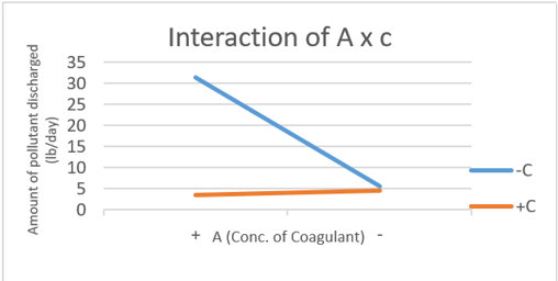
From the graph, we can see that the gradient of -C is negative while +C is positive. They are inversely proportional where low A and high C, reduces the amount of pollutant discharged to about 4 lb/day, which is the lowest obtained from all graphs. Therefore, there's a significant interaction between the two factors.
Lastly, for the interaction for BxC,
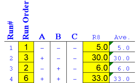
At LOW C,
Average of LOW B = (5 + 30)/2 = 17.5 Average of HIGH B = (6+ 30)/2 = 18
Total effect of B = 18 – 17.5 = 1.5 (increase)
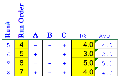
At HIGH C,
Average of LOW B = (4 + 3)/2 = 3.5
Average of HIGH B = (5 + 4)/2 = 4.5
Total effect of B = 4.5 – 3.5 = 1 (increase)

From the graph, we can see that both gradients are negative and are almost parallel. This means both have the same gradient and has the same effect on each other regardless at high or low level. Thus, there is NO interaction between factor B and C.
In conclusion, Factor C, stirrer speed, has the most significant effect on water treatment. However, as Factor C has interaction effects with Factor A, concentration of coagulant added, preforming differently according to the changes of factor A, it is essential to maintain Factor A at a low level for a effective water treatment process.
FRACTIONAL factorial run
For the FRACTIONAL design, I chose the runs 2, 3, 6 and 7, where the high and low levels occur at equal amount of time, giving good statistical proportions.
From the previous data table in excel, I duplicated the same table and deleted all the other runs except the four that I chose for my fractional run.

Just like the full factorial design, with the computed the results, I plotted a graph with the same axis for comparison and determination of results.

It is observable that just like the full factorial design, Factor C contributes the most to the amount of pollutant discharged. It has the steepest curve and the biggest change of -7 as the stirrer speed changes from 400rpm to 200rpm. This suggests that as stirrer speed decrease, the amount of pollutant discharges increases by 14.50. However, a discrepancy occurs when both Factor A and Factor B contributes the second-most to the amount of pollutant discharged in the fractional factorial run.
Factor B has the second-most steep curve and has a change of -5.50 as temperature of treatment decreases from 100 oF to 72 oF. This suggests that as temperature decreases, the amount of pollutant discharged increases by 5.50.
Factor A's curve has a similar steepness to Factor B and a change of +5.50 as concentration of coagulant changes from 2% to 1%. This suggests that as concentration decreases, the amount of pollutant discharged decreases by 5.50.
The final ranking for fractional factorial run are as follows,
Stirrer speed
Concentration of coagulant added and Treatment temperature
The reason for this discrepancy observed is due to the lack of data used during the fractional factorial design. A factorial run is used when there is a lot of data involved and it becomes infeasible to run all the treatments. Hence, DOE is conducted with restricted amount of runs for a realistic approach. However, we initially only had 8 data points to work with. Only going through the runs once is already unreliable as results are subjected to changes between every repeats due to multiple reasons like surrounding environment, thus multiple repeats has to be done for each run to get an average. Therefore, reducing the already very little data given data will further reduce the accuracy of the results, as seen in the fractional run. Fortunately, Factor C came out as the most significant in affecting water treatment for both full and fractional factorial designs, but the fractional run would not be able to deduce the interaction effects due to the lack of data. In conclusion, using a fractional factorial design may not be feasible all the time. We need to be able to critically analyse and decide with what we are given. This is also a crucial skillset as an engineer. For this case study, a FULL factorial design will be more beneficial than a FRACTIONAL factorial design.
Hyperlink to FULL and FRACTIONAL factorial design (Excel Template) :


Comments